Building on my recent project on the source panel method to visualise velocity and pressure distributions in Python, I thought it was reasonable to extend the method to implement the vortex panel method.
Unlike the source panel method, the vortex panel method can be used to visualise the airflow around asymmetric bodies. In order to visualise airflow around asymmetric bodies, the method must be able to produce a non-zero circulation. Circulation is the measure of the net rotational strength of a flow around a closed loop. Mathematically, circulation is the line integral of the velocity field around a closed curve C.
Non-zero circulation implies an asymmetric velocity field around the body, with a component of the flowing around the geometry. This asymmetry leads to a pressure difference between the upper and lower surfaces of the airfoil which is characteristic of a net lift force. This net lift force can be calculated via the Kutta–Joukowski theorem which gives the lift per unit span given the density, the freestream velocity and the net circulation around a closed loop enclosing the geometry.
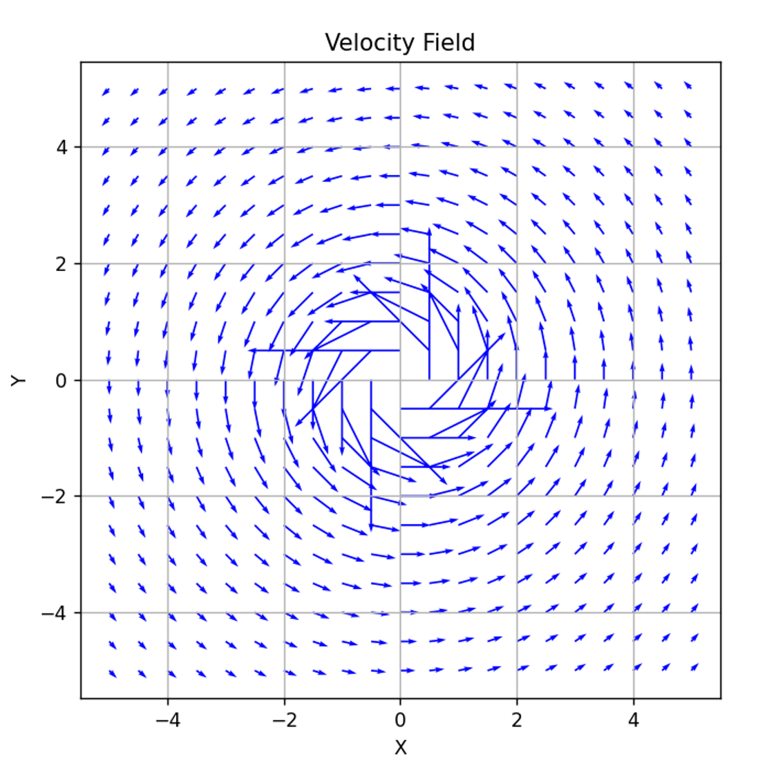
The vortex panel method allows such a non-zero circulation to arise by modelling the airfoil surface as a distribution of vortices along the geometry rather than a distribution of sources. Vortex flow inherently has a non-zero circulation due to how the flow forms; the airflow forms closed swirling streamline around the vortex core, giving a net rotational component when integrated along the contour line. When superimposed with other vortexes, this creates a global circulation around the body.
In practice, this method is very similar to the source panel method: the surface is discretised into a number of small panels, each carrying a vortex of unknown strength. These strengths are solved by enforcing the no-penetration boundary condition at the control points on the surface. A critical additional step, which distinguishes the vortex panel method from the source panel method, is the enforcement of the Kutta condition at the trailing edge to model realistic flow around the trailing edge.
Deriving the Potential Flow equation
This project uses the same NACA airfoil generation and overall code structure as the source panel method implementation. The key difference is how the velocity field is constructed: sources are replaced by vortices when computing the flow.
As in the previous article, the total velocity potential is given by the superposition of the freestream potential and the contributions from the vortices distributed along the panels:
\[ \phi(x,y) = \phi_\infty(x,y) + \sum_{j=1}^{N} \phi_j(x,y) \]
where $\phi_\infty(x,y)$ is the velocity potential from the freestream flow and $\sum_{j=1}^{N} \phi_j(x,y)$ is the addition of the contribution to the potential from each panel.
The velocity potential from the freestream flow is once again $\phi_\infty(x,y) = V_\infty \left( \cos\alpha\, x + \sin\alpha\, y \right)$. as derived in the source panel method article.
To determine the velocity potential due to a vortex, we now consider the flow induced by a two-dimensional point vortex.
We will derive the velocity potential from a point vortex from the velocity equations in polar coordinates. For a point vortex, there is no radial velocity and the tangential velocity is given as a function of the circulation of the vortex.
By definition, the velocity field is related to the velocity potential by $\mathbf{v} = \nabla \phi$. In polar coordinates, this becomes $v_r = \frac{\partial \phi}{\partial r}$ for the radial velocity and $v_\theta = \frac{1}{r}\frac{\partial \phi}{\partial \theta}$ for the tangential velocity. Since the radial velocity is zero, the velocity potential is independent of r and only depends on the angle.
We can then derive the velocity potential using the equation for the tangential velocity:
\[\frac{1}{r}\frac{\partial \phi}{\partial \theta} = \frac{\Gamma}{2\pi r}\]
Rearranging and then integrating with respect to theta yields the velocity potential of a point vortex. This gives us:
\[\phi_v(\theta) = \frac{\Gamma}{2\pi}\theta\]
Thus the velocity potential for uniform freestream flow and the vortices on N panels is given by:
\[\phi(x,y) = \phi_\infty(x,y) + \sum_{j=1}^{N} \phi_j(x,y)\] \[\phi(x,y) = V_\infty \left( \cos\alpha\, x + \sin\alpha\, y \right) + \sum_{j=1}^{N} \frac{\Gamma_j}{2\pi}\,\theta_j\]The equation above would work if the panels are sufficiently small. If the panel lengths are small then the angle between the point (x,y) can be considered to be constant along the entire panel. However, to generalise this code to handle less finely discretised panels, instead of adding the velocity potential induced by the control point of each panel, we’ll adapt the equation to add the velocity potential integrated along each panel. This is written as:
\[ \phi_i = v_\infty \cos (\alpha)x_i + v_\infty \sin(\alpha)y_i +\sum_{j=1}^N-\frac{\gamma_j}{2\pi}\int_j\theta_{ij}ds_j \]Now we have obtained the equation describing the velocity potential at all points in the grid in terms of the circulation of each panel and the characteristics of the freestream velocity. We can now find the velocity in different directions by taking the partial derivative of this velocity potential with respect to that direction.
No-Penetration Condition
With the potential equation we’ll first use it to enforce the no-penetration condition. As in the source panel method, this condition ensures that the flow treats the geometry as a solid body, with zero normal velocity at the airfoil surface and no fluid crossing the boundary. This condition is enforced at the control point of each panel and is calculated by taking the partial derivative of the velocity potential in the normal direction of each panel and then taking the dot product of this with the normal unit vector and equating it is zero:
\[ \frac{\partial \phi}{\partial n_i} = v_\infty \cos \alpha \frac {\partial x_i}{\partial n_i} + v_\infty \sin \alpha \frac {\partial y_i}{\partial n_i} + \sum_{j=1}^{N} -\frac {\gamma_j}{2\pi} \int_j \frac {\partial \theta_{ij}}{\partial n_i} ds_j \]First, let’s examine the first two expressions in this addition which come from the velocity potential of the uniform flow:
\[ v_\infty \cos \alpha \frac {\partial x_i}{\partial n_i} + v_\infty \sin \alpha \frac {\partial y_i}{\partial n_i} \]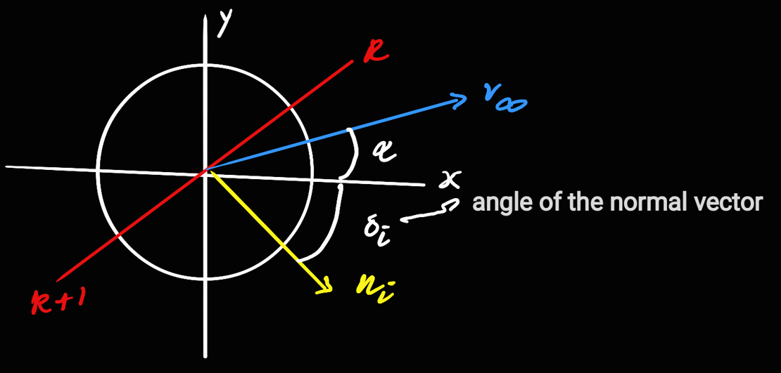
As shown in the drawing above, we can make some relations between the angles involved in each panel. Given the angle of attack is at $\alpha$ radians and the normal vector $\n_i$ is at $\sigma_i$ radians measured from the positive x-axis, we can write the angle from the freestream velocity to the normal vector as $\sigma_i - \alpha$. We’ll call this angle $\beta_i$ for panel i.
Now we can write the partial derivatives in the first part of the expression in terms of the angle $\sigma_i$.
\[\frac {\partial x_i}{\partial n_i} = \cos (\sigma_i)\]
\[\frac {\partial y_i}{\partial n_i} = \sin (\sigma_i)\]
Hence using the cosine addition formula we can write the expression in the form of \beta_i:
\begin{align} v_\infty(\cos\alpha \cos\sigma_i + \sin\alpha \sin\sigma_i) &= v_\infty \cos(\alpha - \sigma_i) \\ &= v_\infty \cos \beta_i \end{align}
This respresents the freestream contribution to the normal velocity at control point $i$. Now, we can enforce the no-penetration condition in a similar way to how we did for the source panel method by equating the equation above to 0.
\[\frac{\partial \phi}{\partial n_i} = 0, \quad i=1,2,\dots,N\]
\[v_\infty \cos\beta_i - \sum_{j=1}^{N} \frac{\gamma_j}{2\pi} \int_j \frac{\partial \theta_{ij}}{\partial n_i} \, ds_j = 0, \quad i = 1,2,\dots,N\]
\[\begin{bmatrix} \frac{1}{2\pi} \int_1 \frac{\partial \theta_{11}}{\partial n_1} ds_1 & \frac{1}{2\pi} \int_2 \frac{\partial \theta_{12}}{\partial n_1} ds_2 & \cdots & \frac{1}{2\pi} \int_N \frac{\partial \theta_{1N}}{\partial n_1} ds_N \\ \frac{1}{2\pi} \int_1 \frac{\partial \theta_{21}}{\partial n_2} ds_1 & \frac{1}{2\pi} \int_2 \frac{\partial \theta_{22}}{\partial n_2} ds_2 & \cdots & \frac{1}{2\pi} \int_N \frac{\partial \theta_{2N}}{\partial n_2} ds_N \\ \vdots & \vdots & \ddots & \vdots \\ \frac{1}{2\pi} \int_1 \frac{\partial \theta_{N1}}{\partial n_N} ds_1 & \frac{1}{2\pi} \int_2 \frac{\partial \theta_{N2}}{\partial n_N} ds_2 & \cdots & \frac{1}{2\pi} \int_N \frac{\partial \theta_{NN}}{\partial n_N} ds_N \end{bmatrix} \begin{bmatrix} \gamma_1 \\ \gamma_2 \\ \vdots \\ \gamma_N \end{bmatrix} = \begin{bmatrix} v_\infty \cos\beta_1 \\ v_\infty \cos\beta_2 \\ \vdots \\ v_\infty \cos\beta_N \end{bmatrix}\]
In the source panel method, the influence of a panel's strength on itself was equal to half of the panel's source strength. In the vortex panel method, however, a vortex has no influence on itself and thus the panel influence integral equates to zero along the diagonal of this linear system of equations. This gives us:
\[\begin{bmatrix} 0 & \frac{1}{2\pi} \int_2 \frac{\partial \theta_{12}}{\partial n_1} ds_2 & \cdots & \frac{1}{2\pi} \int_N \frac{\partial \theta_{1N}}{\partial n_1} ds_N \\ \frac{1}{2\pi} \int_1 \frac{\partial \theta_{21}}{\partial n_2} ds_1 & 0 & \cdots & \frac{1}{2\pi} \int_N \frac{\partial \theta_{2N}}{\partial n_2} ds_N \\ \vdots & \vdots & \ddots & \vdots \\ \frac{1}{2\pi} \int_1 \frac{\partial \theta_{N1}}{\partial n_N} ds_1 & \frac{1}{2\pi} \int_2 \frac{\partial \theta_{N2}}{\partial n_N} ds_2 & \cdots & 0 \end{bmatrix} \begin{bmatrix} \gamma_1 \\ \gamma_2 \\ \vdots \\ \gamma_N \end{bmatrix} = \begin{bmatrix} v_\infty \cos\beta_1 \\ v_\infty \cos\beta_2 \\ \vdots \\ v_\infty \cos\beta_N \end{bmatrix}\]
Now that we’ve simplified the velocity potential equation and made the linear system of equations, we'll move on to simplifying the integral part of the expression.
Deriving the panel influence integral
In this section, we will derive the panel influence integral $\int_j \frac {\partial \theta_{ij}}{\partial n_i} ds_j$ which respesents the integral of the partial derivative of the angle at panel $i$ from panel $j$ with respect to the normal vector of that panel.
Let us consider a point on panel $j$ where s is the parameter that defines the distance along the panel j.
\[\theta(s) = tan^{-1} (\frac{y(s) - y}{x(s) - x}) \]
Let us define $u = x-x_i, v = y-y_i$ so that $\theta = \tan^{-1}\!\left(\frac{v}{u}\right)$.
Using the chain rule, we can find expressions for the partial derivatives of the angle with respect to the directions x and y in terms of u and v.
\[ \frac{\partial \theta}{\partial x} = \frac{1}{1+(v/u)^2} \left( -\frac{v}{u^2} \right) = -\frac{v}{u^2+v^2} \] \[ \frac{\partial \theta}{\partial y} = \frac{1}{1+(v/u)^2} \left( \frac{1}{u} \right) = \frac{u}{u^2+v^2} \]
We can then substitute u and v back into the equation to get the following equation: \[ \nabla \theta = \begin{pmatrix} -\dfrac{y-y_i}{(x-x_i)^2+(y-y_i)^2} \\ \phantom{-}\dfrac{x-x_i}{(x-x_i)^2+(y-y_i)^2} \end{pmatrix} = \frac{1}{r^2} \begin{pmatrix} -(y-y_i) \\ \phantom{-}(x-x_i) \end{pmatrix} \] \[ r^2 = (x-x_i)^2+(y-y_i)^2 \]
Now that we have the partial derivatives of the angle with respect to x and y, we can relate this to the normal vector through the relation between the angle $\phi_i$ and the unit normal vector. The angle of the normal is at $\phi_i + \frac{\pi}{2}$. Hence the x component of the normal unit vector is $\cos (\phi_i + \frac{\pi}{2}) = -\sin(\theta)$ and the y component of the normal unti vector is $\sin(\phi_i + \frac{\pi}{2}) = \cos(\theta)$.
The unit normal at control point $i$ is \[ \hat{\mathbf{n}}_i = \begin{pmatrix} -\sin\phi_i \\ \cos\phi_i \end{pmatrix} \].
Thus, we can find the partial derivative of the angle with respect to the normal vector by taking the dot product between the gradient of the angle and the normal unit vector. This gives us:
\[ \frac{\partial \theta}{\partial n_i} = \nabla\theta \cdot \hat{\mathbf{n}}_i = \frac{ -(y-y_i)(- \sin)\phi_i + (x-x_i)\cos\phi_i }{r^2} \]
Now we'll use the parameter $s$ we defined before to rewrite $(x-x_i)$ and $(y-y_i)$ as an expression of constant terms within the grid.
Panel $j$ is parameterised by $x(s)=x_j+s\cos\phi_j$ and $y(s)=y_j+s\sin\phi_j$. As $(x-x_i)$ and $(y-y_i)$ are functions of x and y, we can replace x and y with these parameterised form and then substitute these variables into the numerator in the previous equation we obtained for $\frac{\partial \theta}{\partial n_i}$:
\[ x-x_i = (x_j-x_i)+s\cos\phi_j, y-y_i = (y_j-y_i)+s\sin\phi_j \]
\[\frac{ -(y-y_i)(- \sin\phi_i) + (x-x_i)\cos\phi_i }{r^2} = \frac{[(y_j-y_i)+s\sin\phi_j]sin \phi_j + [(x_j-x_i)+s\cos\phi_j]cos \phi_j]}{r^2}\]
This is equal to $\frac{\partial \theta}{\partial n_i} = \frac{s\cos(\phi_i - \phi_j) + (x_j-x_i)\cos(\phi_i) + (y_j - y_i)sin(\phi_i)}{r^2}$
The denominator $r^2$ is equal to $(x_j-x_i)+s\cos(\phi_j)^2 + (y_j-y_i)+s\sin(\phi_j)^2$. Expanding out the brackets gives us $s^2 - 2s(x_i-x_j)\cos\phi_j - (y_i-y_j)\sin\phi_j + (x_j-x_i)^2 + (y_j-y_i)^2$.
The panel influence integral becomes $\frac{\partial \theta}{\partial n_i} = \int_0^{S_j} \frac{Cs + D}{s^2 + 2As + B} \, ds$
A bit of rearranging gives us:
\[ \begin{aligned} \frac{\partial \theta}{\partial n_i} &= \frac{C}{2} \int_0^{S_j} \frac{2s+2A}{s^2+2As+B}\, ds \\ &\quad +(D-AC) \int_0^{S_j} \frac{ds}{s^2+2As+B} \end{aligned} \]
We can then evaluate both integrals separately. The first integrand can be written as the derivative of $ln(s^2+2As+B)$. The second integrand cannot be written in the same way as the numerator consists of only the differential. Thus we cannot apply the reverse chain rule here and instead we'll complete the square to put the integrand in the form of the derivative of an arctan function.
\[ s^2+2As+B=(s+A)^2+E^2, \quad E=\sqrt{B-A^2} \] \[ \int \frac{ds}{(s+A)^2+E^2} = \frac{1}{E} \tan^{-1}\!\left(\frac{s+A}{E}\right) \]
Thus we can rewrite the full integral as:
\[ {\frac{\partial \theta}{\partial n_i} = \frac{C}{2} \ln\!\left( \frac{S_j^2+2AS_j+B}{B} \right) + \frac{D-AC}{E} \left[ \tan^{-1}\!\left(\frac{S_j+A}{E}\right) - \tan^{-1}\!\left(\frac{A}{E}\right) \right] } \]
where the constants A, B, C, D and E are defined as follows:
$A = (x_j - x_i)\cos\phi_j + (y_j - y_i)\sin\phi_j $
$B = (x_j - x_i)^2 + (y_j - y_i)^2$
$C = \cos(\phi_i - \phi_j)$
$D = (x_j - x_i)\cos\phi_i + (y_j - y_i)\sin\phi_i$
$E = \sqrt{B - A^2}$
Gladly, we don't need to worry about integrating this by hand as we are coding this. Thus, all we'll do is loop through each of the panels and calculate the panel influence integrals for each panel:
for i in range(num_pan):
        dx = XB[i+1] - XB[i]
        dy = YB[i+1] - YB[i]
        s_panels[i] = (dx**2+dy**2)**0.5 #length of panel

        phi_panels[i] = np.arctan2(dy, dx)
        if phi_panels[i] < 0:
            phi_panels[i] += 2*np.pi

        sigma_panels[i] = np.arctan2(dy, dx) + np.pi/2
        beta_panels[i] = sigma_panels[i] - V_a

    def computeintegral(i, j): #the influence ON panel i FROM panel j
        A = -1*(XC[i]-XB[j])*np.cos(phi_panels[j]) - (YC[i]-YB[j])*np.sin(phi_panels[j])
        B = (XC[i]-XB[j])**2 + (YC[i]-YB[j])**2
        C = - np.cos(phi_panels[i] - phi_panels[j])
        D = (XC[i]-XB[j])*np.cos(phi_panels[i]) + (YC[i]-YB[j])*np.sin(phi_panels[i])
        E = (B - A**2)**0.5
        if (E == 0 or np.iscomplex(E) or np.isnan(E) or np.isinf(E)):
             I = 0                                                    # if E term is invalid
        else:
            I = C/2*np.log(((s_panels[j])**2 + 2*A*s_panels[j] + B)/B) + ((D - A*C)/E)*(np.arctan2((s_panels[j]+A), E) - np.arctan2(A, E))

        return I
Let's start with the Kutta condition.
Kutta Condition
The Kutta condition is a condition that ensures a physically realistic flow around sharp trailing edges. Without the Kutta condition, the circulation around the airfoil can take any value. As Laplace's equation is linear, any constant circulation added around a closed contour still satisfies Laplace's equation. Thus, without an additional physical condition, the solution acquired is not unique. At the sharp trailing edge, without the Kutta condition, the velocity tends to infinity as the flow tries to turn around the corner. The Kutta condition enforces that the flow leaves the trailing edge smoothly such that the velocity is finite and the upper and lower surface evlocities are equal. Thus the trailing edge acts like a stagnation point. The tangential velocity at this point is porportional to the sum of the vortex strengths at the upper and lower panels and thus the sum of the two panels connected to this point must equal zero:
\[\gamma_1 + \gamma_N = 0\]
The code to enforce the Kutta condition is extremely simple; all we need to do is replace the last row in the array with an equation that represents the condition. We must replace one of the equations rather than add another equation in order to ensure the system is not over-constrained.
B_matrix = -1*V_fs*2*np.pi*np.cos(beta_panels).reshape(num_pan, 1)
    B_matrix[-1] = 0

    A_matrix = np.zeros((num_pan, num_pan))
    for i in range(num_pan): #analysing the ith panel
        for j in range(num_pan): #the influence of the jth panel on the ith panel
            if i == j:
                A_matrix[i, j] = 0
            else:
                A_matrix[i, j] = -1*computeintegral(i, j)
    A_matrix[-1] = np.zeros (num_pan)
    A_matrix[-1, :] = 0
    upper_TE = nU - 1
    lower_TE = nU

    A_matrix[-1][upper_TE ] = 1
    A_matrix[-1][lower_TE ] = 1

Vsource_strengths = np.linalg.solve(A_matrix, B_matrix)\[V_{x,P} = \frac{\partial \phi_P}{\partial x_P} = V_\infty \cos \alpha + \sum_{j=1}^{N} -\frac{\gamma_j}{2\pi} \int_j \frac{\partial \theta_{ij}}{\partial x_P} \, ds_j\]
\[V_{y,P} = \frac{\partial \phi_P}{\partial y_P} = V_\infty \sin \alpha + \sum_{j=1}^{N} -\frac{\gamma_j}{2\pi} \int_j \frac{\partial \theta_{ij}}{\partial y_P} \, ds_j\]
\[\int_j \frac{\partial \theta_{ij}}{\partial x_P} \, ds_j = \frac{C_x}{2} \ln \left( \frac{s_j^2 + 2 A s_j + B}{B} \right) + \frac{D_x - A C_x}{E} \left[ \tan^{-1} \left( \frac{s_j + A}{E} \right) - \tan^{-1} \left( \frac{A}{E} \right) \right]\]
\[\int_j \frac{\partial \theta_{ij}}{\partial y_P} \, ds_j = \frac{C_y}{2} \ln \left( \frac{s_j^2 + 2 A s_j + B}{B} \right) + \frac{D_y - A C_y}{E} \left[ \tan^{-1} \left( \frac{s_j + A}{E} \right) - \tan^{-1} \left( \frac{A}{E} \right) \right]\]
Where:
$A = -(x_P - x_j) \cos \phi_j - (y_P - y_j) \sin \phi_j, \quad$
$B = (x_P - x_j)^2 + (y_P - y_j)^2$
$C_x = \sin \phi_j, \quad D_x = -(y_P - y_j), \quad$
$C_y = -\cos \phi_j, \quad D_y = x_P - x_j, \quad$
$E = \sqrt{B - A^2}$
In code, to plot the velocity at each point in the grid, this becomes:
Vsource_strengths, XC, YC, s_panels, XB, YB, phi_panels = source_analyse_naca(nacadigits, V_fs, V_a)
    dx = 0.025
    XXX, YYY =  np.meshgrid(np.arange(-1, 2+dx, dx), np.arange(-0.5, 0.5+dx, dx)) #the underlying gridpoints

    U = np.zeros(np.shape(XXX)) #x direction
    V = np.zeros(np.shape(XXX)) #y direction

    XC = XC.flatten()           #shape: (N_panels,)
    YC = YC.flatten()
    xj = XB[:-1].flatten()
    yj = YB[:-1].flatten()
    s = s_panels.flatten()
    phi = phi_panels.flatten()

    #finding the distances
    dx = XXX[:, :, None] - xj[None, None, :]
    dy = YYY[:, :, None] - yj[None, None, :]

    #terms for the geometric integral
    A = -dx * np.cos(phi[None, None, :]) - dy * np.sin(phi[None, None, :])
    B = dx**2 + dy**2
    Cx = np.sin(phi[None, None, :])
    Cy = -np.cos(phi[None, None, :])
    Dx = dx
    Dy = -dy
    E = np.sqrt(np.maximum(B - A**2, 1e-12))  # avoid sqrt of negative

    numerator = s[None, None, :]**2 + 2*A*s[None, None, :] + B
    ratio = np.maximum(numerator / B, 1e-12)
    log_term = np.log(ratio)
    atan_term = np.arctan2(s[None, None, :] + A, E) - np.arctan2(A, E)

    gamma = Vsource_strengths.flatten()
    U = np.sum(gamma[None, None, :] * (0.5 * Cx * log_term + ((Dx - A * Cx) / E) * atan_term) / (2*np.pi), axis=2)
    V = np.sum(gamma[None, None, :] * (0.5 * Cy * log_term + ((Dx - A * Cx) / E) * atan_term) / (2*np.pi), axis=2)

    U += V_fs * np.cos(V_a) #add the freestream velocity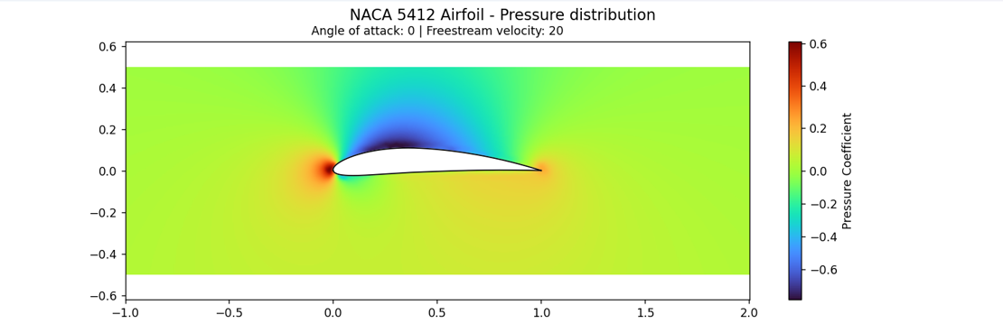
V += V_fs * np.sin(V_a) #PRESSURE DISTRIBUTION PLOT
rho = 1.225
P_inf = 0
P = P_inf + 0.5 * rho * (V_fs**2 - speed_fine**2)
Cp = 1 - (speed_fine / V_fs)**2
fig, ax = plt.subplots(figsize=(12,4))
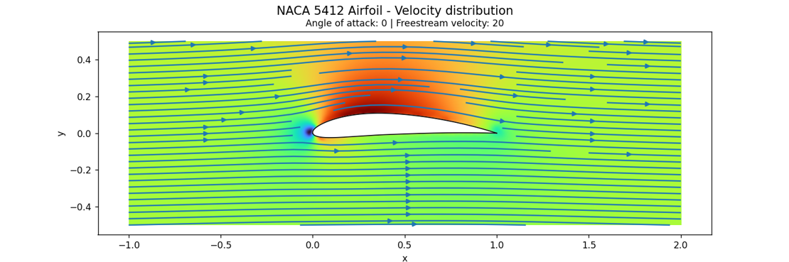
Now, we're mostly done! Here are some plots generated by the program below:
Calculating Lift
At the start of the article, I provided the equation relating the lift per unit span and the circulation of the velocity field:
\[L' = \rho v_{\infty} \Gamma\]
Thus, to calculate the lift per unit span we'll need to first numerically calculate the circulation. Circulation is given by$ \Gamma = \oint_C \mathbf{v} \cdot d\mathbf{l}$.
The most apparent way to calculate this is to use the velocity field we have calculated and integrate the velocity along a closwed contour that fllows the shape of an ellipse that encloses the airfoil body.
Although this is a conceptually correct way to caluclate circulation, the velocity is only caluated at the panel control points as well as a mesh of points in the field of view. However, the discretised ellipse will inevitably contain boundary points for integration that lie outside this collection of points. Thus to calculate the velocity at these points we would have to interpolate the velocity between the nearby points which could gain some inaccuracy across the integral.
Instead, we can use Stoke's Theorem to rewrite the closed contour integral to a surface integral instead. Stoke's Theorem states that for any smooth vector field:
\[\oint_{\partial S} \mathbf{F} \cdot d\mathbf{l} = \iint_{S} (\nabla \times \mathbf{F}) \cdot \mathbf{n}\, dS\]
Thus, for our velocity field from our vortex flow, we can write the circulation as the flux of the vorticity through ther surface. This is written below as the surface integral of the vorticity over the area enclosed by the contour.
\[\Gamma = \oint_C \mathbf{v} \cdot d\mathbf{l} = \iint_A (\nabla \times \mathbf{v}) \cdot \mathbf{n}\, dA\]
As the flow formed by the vortex panel method satisfies Laplace's equation, the curl of the velocity field and the divergence of the velocity field are both equal to zero. Thus, in terms of the fluid flow, the fluid is both incompressible and irrotational. The term we are integrating across the surface, which is $\nabla \times \mathbf{v}$, is equivalent to the vorticity of the flow at that point $\omega$. However, as we discussed, for potential flow $\omega = 0$ everywhere in the fluid.
At first glance, this seems to imply that the circulation must also be zero. Yet we know that the circulation around an airfoil cannot be zero if it is generating lift. It is now important to realise that all the vorticity is concentrated on the sirfoil surface itself (in the form of the vortices distributed along each panel). The summation of the vorticity along the airfoil boundary allows the cirulation to be non-zero even through the flow elsewhere is irrotational. As we used $\gamma_j$ to represent the vortex strength per unit length along the panel, the circulation can be expressed as this integral along the airfoil:
\[\Gamma = \int_{surface}\gamma(s)ds\]
This is represented very simply in the code:
    Gamma = np.sum(vortex_strengths * s_panels)
    print (Gamma)
We can then use the equation $L' = \rho v_{\infty} \Gamma$ to calculate the lift per unit span experienced by the airfoil at the freestream velocity $v_{\infty}$.
Overall, the vortex panel method is more physically accurate than the source panel method as it can produce physical approximations for asymmetric airfoils by using vortices instead of sources which then provide a way to calculate both the lift and circulation of the airfoil. However, the method still does not account for viscosity, which means it cannot capture effects like boundary layers or flow separation. As a result, while it gives a good estimate of lift and circulation, it tends to overpredict performance compared to what would actually occur in real airflow.