Recently, I decided I wanted to build a 2D airflow analyser to visualise flows over NACA airfoils.
For reference, the flows my program produced at the end of this project look like this:
My first instinct when approaching this project was to write a program to numerically solve the Navier Stokes equations. In principle, this would give a full velocity and pressure field application to various flow types (compressible, viscous, unsteady etc.).
In practice, however, this method requires a full CFD infrastructure: generating a mesh body, discretizing the equations, coupling the pressure and velocity and even modelling turbulence. These steps are computationally intensive and for the purpose of analysing 2D airflows at small angles of attack, the dominant features of the flow can be captured using panel methods and potential flow theory.
Potential flow theory is a simplified model which describes flows that are inviscid, incompressible, and irrotational. Under these assumptions, the velocity field $v=\nabla\phi$ can be described as the gradient of a scalar velocity potential $\phi$ where $\nabla$ represents the vector of partial derivatives $\nabla = \left[\frac{\partial}{\partial x}, \frac{\partial}{\partial y} \right]$.
Furthermore, as the flow is incompressible, the divergence of the velocity field is zero $\nabla \cdot v = 0$. Substituting the potential into the continuity equation, we arrive at Laplace’s equation $\nabla^2 \phi = 0$.
This governing equation is linear, so the principle of superposition allows complex flow fields to be constructed by summing together the potentials from elementary flows that collectively describe the flow field.
In the source panel method, the geometry is discretised into straight-line panels, each carrying a constant source strength distributed over its length. A source is a radial flow of some volume per second. In our 2D simulation, this becomes the flow of area/second. Solving for these source strengths to satisfy the boundary conditions on the surface transforms flow visualisation into a solvable system of linear equations.
NACA profiles
Note: It is important to mention that the source panel method on its own assumes the body is symmetric to produce meaningful analysis. For cambered airfoils, this method alone cannot capture the generation of lift as sources produce no circulation. Additional elements, such as vortex panels, are required to model asymmetric geometries accurately.
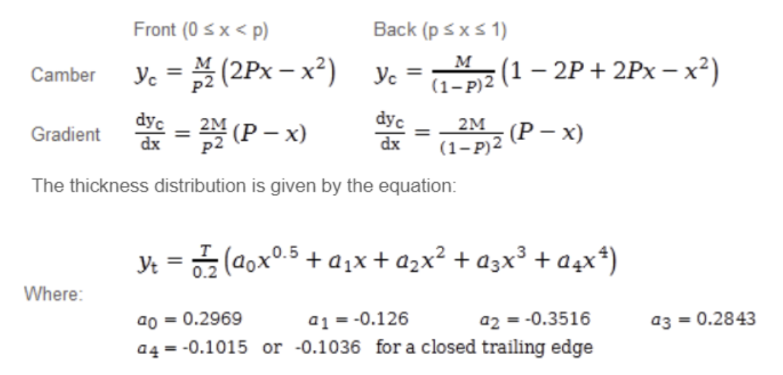
NACA 4-digit airfoils are constructed by four digits, each representing a specific geometric parameter.
Once these parameters are specified, the airfoil geometry is generated using preset analytical equations that define the x and y values of the camber line and thickness along the chord.
The equation of the camber line is a piecewise equation with separate functions for x values before and after the maximum camber point.
The gradient of the camber line allows us to calculate the angle between the positive x axis and the camber line which can be used to calculate the coordinates for the upper and lower surfaces of the airfoil.
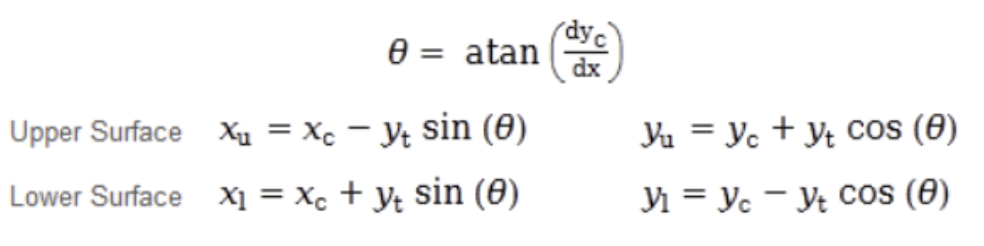
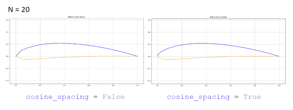
Given these equations, a natural approach is to evaluate the upper and lower surface coordinates at uniformly spaced chordwise intervals. However, this fails to account for variation in the curvature of the airfoil along the chord: near the leading and trailing edges the gradients are large and higher resolution is required, whereas around mid-chord the geometry is relatively flat and fewer panels are sufficient.
A better way to plot such geometries is to use cosine spacing. Cosine spacing is a method that uses a non-uniform distribution of points along the chord, clustering them near the leading and trailing edges where the curvature is highest. This is achieved by defining points in terms of an angle $\theta$ varying at regular intervals from $0$ to $\pi$ and then mapping them to the chord using the formula $x = \frac{1}{2}(1 - cos \theta)$.
Code: Plotting NACA Profiles
The code below used the equations above to find the equation of the camber line and then make four 2D arrays with the x and y coordinates of each of the points on the upper and lower surfaces, represented by xu,xl,yl,yu.
def naca(nacadigits, n_points = 200, cosine_spacing = True):
    chord = 1
    num_pan = n_points - 1
    m = int(nacadigits[0])/100.0
    p = int(nacadigits[1])/10.0
    t = int(nacadigits[-2:])/100.0


    if cosine_spacing == False:
        xc = np.linspace(0, 1, n_points)
    else:
        angles = np.linspace (0, np.pi, n_points)
        xc = (1-np.cos(angles))/2


    if m == 0:
        yc = np.zeros_like(xc)
        dyc_dx = np.zeros_like(xc)
    else:
        yc = np.where(
            xc < p,
            m/(p**2)*(2*p*xc - xc**2),
            m/((1-p)**2)*(1 - 2*p + 2*p*xc - xc**2)
        )
        dyc_dx = np.where(
            xc < p,
            2*m/(p**2)*(p - xc),
            2*m/((1-p)**2)*(p - xc)
        )
    theta = np.arctan(dyc_dx)


    yt = t/0.2 * (0.2969*xc**0.5 - 0.126*xc - 0.3516*xc**2 + 0.2843*xc**3 -0.1036*xc**4)


    xu = xc - yt*np.sin(theta)
    xl = xc + yt*np.sin(theta)
    yu = yc + yt*np.cos(theta)
    yl = yc - yt*np.cos(theta)


    return xu, xl, yu, yl
The function naca_plot(digits) uses matplotlib to show these equations. Prior to plotting the equations, however, the arrays x_polygon and y_polygon are created; these are the two coordinate arrays defining a closed loop around the airfoil surface.
def naca_plot (digits):
    #plt.figure(figsize=(10, 4))
    xu, xl, yu, yl = naca(digits)
    x_polygon = np.concatenate([xu, xl[::-1]])  # upper, then lower
    y_polygon = np.concatenate([yu, yl[::-1]])


    plt.fill(x_polygon, y_polygon, color=(1, 1, 1))
    plt.plot(xu, yu, label='Upper surface', linewidth=1, color='black')
    plt.plot(xl, yl, label='Lower surface', linewidth=1, color='black')
    plt.title(f"NACA {digits} Airfoil")
    plt.grid(True)
    plt.axis('equal')
    plt.show()
Deriving the Velocity Potential Equation
To derive the velocity potential at all grid points in our space, we’ll begin by deriving the velocity potential due to the freestream velocity and then superimposing the velocity potentials due to other sources.
As we concluded that Laplace’s equation was linear, this becomes: \[\phi(x, y) = \phi_\infty(x, y) + \sum^N_{j = 1} \phi_j(x, y)\]
where $\phi_\infty(x, y)$ is the velocity potential from the freestream flow and $\sum^N_{j = 1} \phi_j(x, y)$ is the addition of the contribution to the potential from each panel.
Let us first find $\phi_\infty(x, y)$. If we consider the freestream flow $V_\infty$ to have an angle of attack of $\alpha$, the velocity components are $v_{x, \infty} = V_\infty \cos \alpha$ in the x direction and $v_{y, \infty} = V_\infty \sin \alpha$ in the y direction. From our previous definition of the velocity as the gradient of the scalar velocity potential field, we get that the velocity in each respective direction is the partial derivative of the potential with respect to a unit distance in this direction.
For our x and y directions, this gives us two equations describing the freestream velocity potential $v_{x, \infty} = \frac{\partial \phi_\infty}{\partial x} = V_\infty \cos \alpha$ and $v_{y, \infty} = \frac{\partial \phi_\infty}{\partial y} = V_\infty \sin \alpha$.
By integrating the first equation with respect to x, we get $\phi_\infty = V_\infty \cos \alpha \times x + f(y)$.
If we plug this representation of the potential of the freestream flow into the second equation, we get $f'(y) = V_\infty \sin \alpha$. Hence, $f(y) = V_\infty \sin \alpha \times y$
Thus, we have derived the velocity potential from the freestream flow to be:
\[\phi_\infty(x,y) = V_\infty \cos \alpha \times x + V_\infty \sin \alpha \times y\]
We can now consider the velocity potential from a single 2D source with source strength $\sigma_j$ at position $(x_j, y_j)$. The source strength $\lambda_j$ has units $m^3/s$ for 3D geometries. For this 2D visualisation, I’ll use $\sigma_j$ to represent the source strength per unit depth. I like to think of this as the area leaving the point per second. Hence at a distance $r$ away from the source, the circumference of the flow at this point is $2\pi r$ and hence the velocity of the flow in the radial direction is $v_r = \frac{\sigma_j}{2\pi r}$.
As $\frac{\partial \phi_j}{\partial r} = \frac{\sigma_j}{2\pi r}$, we can obtain the velocity potential due to the single source by integrating this with respect to$r$, giving $\phi_j = \frac{\sigma_j}{2\pi} \ln r + C$ where we can set C to zero as only gradients matter in the velocity potential.
We have now derived the equations needed to describe the velocity potential field (the equation we included at the start) in terms of x and y:
\[\phi(x,y) = V_\infty \left( \cos \alpha , x + \sin \alpha , y \right) + \sum_{j=1}^{N} \frac{\sigma_j}{2\pi} \ln \left( (x - x_j)^2 + (y - y_j)^2 \right)\]
Deriving the Velocity Equation
Now that we have an equation describing the velocity potential at any point in space in terms of x and y, we can now once again use $\mathbf{v} = \nabla \phi$ to find the velocity in each axis by integrating the equation with respect to $x$ for $v_x$ and then with respect to $y$ for $v_y$.
This gives us:
\[
v_x = V_\infty \cos \alpha + \sum_{j=1}^{N} \frac{\sigma_j}{2\pi} \frac{x - x_j}{(x - x_j)^2 + (y - y_j)^2}
\] \[
v_y = V_\infty \sin \alpha + \sum_{j=1}^{N} \frac{\sigma_j}{2\pi} \frac{y - y_j}{(x - x_j)^2 + (y - y_j)^2}
\]
No-penetration boundary condition
Once the velocity potential and velocity equations are defined, the next (and most crucial) step in the source panel method is to enforce the no-penetration boundary condition. Physically, this condition states that the fluid cannot flow through a solid surface. This essentially means that when we compute the velocity at the points on the airfoil geometry, the velocity must be tangent to the surface - any perpendicular component of velocity on the surface signifies air flowing into the airfoil and would violate the no-penetration condition. This condition is enforced at the midpoint of each panel, called the control point.
Mathematically, this is expressed very simply $v(x_i, y_i)\cdot n_i=0$ where $n_i$ is the outward-pointing normal vector of the ith panel. In Python, the normal vector for each panel can be computed from the panel angle phi_panels.
We calculate the angle of the panels from the positive x axis by using dx and dy and then add $2\pi$ to ensure that all angles are positive.
        phi_panels[i] = np.arctan2(dy, dx)
        if phi_panels[i] < 0:
            phi_panels[i] += 2*np.pi
Then, due to the orientation of our panels we can simply add \frac{\pi}{2} to get the angle of the normal of each panel.
Note: beta_panels is the angle of the panel relative to the freestream velocity.
    for i in range(num_pan):
        dx = XB[i+1] - XB[i] #x length of panel
        dy = YB[i+1] - YB[i] #y length of panel
        s_panels[i] = (dx**2+dy**2)**0.5


        phi_panels[i] = np.arctan2(dy, dx)
        if phi_panels[i] < 0:
            phi_panels[i] += 2*np.pi


        sigma_panels[i] = np.arctan2(dy, dx) + np.pi/2 #panel normals
        beta_panels[i] = sigma_panels[i] - V_a #relative to freestream
For more intuition on the angles, I drew this example at the $i$th panel: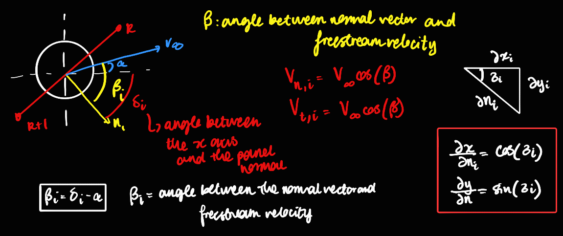
Forming the Linear System
In order to form our system of equations, we’ll enforce the no-penetration boundary condition at each panel. In a geometrical system of N panels, we now have N equations. If we think about our unknowns, we also have N unknowns which are the source strengths of each panel (these are chosen based on the no-penetration condition). We’ll use this to generate a linear system of equations and then use numpy’s linear algebra features to solve this.
As derived before: $v_i = v_\infty + \sum_{j=1}^{N} v_{ij}$ where $v_i$ is the vector of the velocity at the $i$ th panel and $v_{ij}$ is the vector of the velocity induced at panel $j$ due to the control point on the $i$ th panel.
Using the angle diagram above and our velocity equation, I’ve derived the normal velocity on the $i$ th panel below:
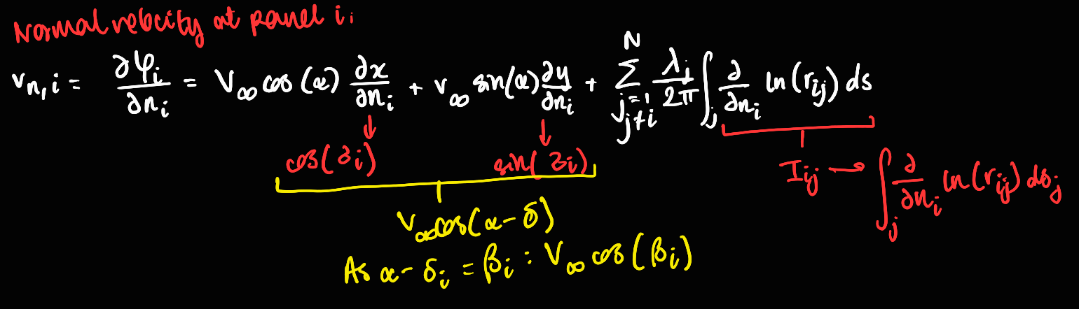
Now we have the equation $V_\infty \cos \beta_i + \sum_{j=1}^{N} ( \mathbf{v}_{ij} \cdot \mathbf{n}_i ) = 0$.
In our linear system of equations, we are aiming to get a matrix equation that can be solved numerically in the form $A \sigma = B$ where $A$ is the N by N influence coefficient matrix, $\sigma$ is the N by 1 matrix of the source strengths and $B$ is the N by 1 matrix of the negative of the normal of the freestream flow at each panel.
For example:
$A_{ij}$ is the normal velocity at the control point $i$ induced by a unit-strength source on panel $j$.
$B_i$ is $B_i = -V \infty \cos \beta_i$
Finding an analytical expression for $A_{ij}$
This integral is standard in low-speed incompressible aerodynamics textbooks e.g Katz & Plotkin, Low-Speed Aerodynamics
I’ve implemented the standard equation for computing influence coefficients into the code below:
 def computeInfCoeff(i, j):
        A = -1*(XC[i]-XB[j])*np.cos(phi_panels[j]) - (YC[i]-YB[j])*np.sin(phi_panels[j])
        B = (XC[i]-XB[j])**2 + (YC[i]-YB[j])**2
        C = np.sin(phi_panels[i] - phi_panels[j])
        D = -1*(XC[i]-XB[j])*np.sin(phi_panels[i]) + (YC[i]-YB[j])*np.cos(phi_panels[i])
        E = (B - A**2)**0.5
        if (E == 0 or np.iscomplex(E) or np.isnan(E) or np.isinf(E)):
             I = 0                                                    # if E term is invalid
        else:
            I = C/2*np.log(((s_panels[j])**2 + 2*A*s_panels[j] + B)/B) + ((D - A*C)/E)*(np.arctan2((s_panels[j]+A), E) - np.arctan2(A, E))


        return I
We can now assemble our matrix to find the source strengths at each of the points:
B = np.zeros((num_pan, 1))


    for i in range(num_pan):
        B[i] = -1*V_fs*2*np.pi*np.cos(beta_panels[i])


    A = np.zeros((num_pan, num_pan))
    for i in range(num_pan): #analysing the ith panel
        for j in range(num_pan): #the influence of the jth panel on the ith panel
            if i == j:
                A[i, j] = np.pi
            else:
                A[i, j] = computeInfCoeff(i, j)


    source_strengths = np.linalg.solve(A, B)
Now, the velocity potential field around the airflow is fully determined and we can now use this velocity potential to find the velocity at all points in the grid.
It’s often useful to check that the total source strength is very close to 0; we do not want to be creating extra material:
  for i in range(num_pan):
        total += source_strengths[i]*s_panels[i] #total source strength
Finding the induced velocity on the grid
For each panel $j$, the induced velocity on all points is computed using the same geometric integral we discussed when forming $A_{ij}$. The only difference is that instead of computing the velocity at the point at which the panel is, we will now be computing the velocity at each point in the grid. As this is a lot of computation, it is important to vectorise this code through NumPy arrays for quicker results.
The code for this is below:
    U = np.zeros(np.shape(XXX)) #x direction
    V = np.zeros(np.shape(XXX)) #y direction


    XC = XC.flatten()           #shape: (N_panels,)
    YC = YC.flatten()
    xj = XB[:-1].flatten()
    yj = YB[:-1].flatten()
    s = s_panels.flatten()
    phi = phi_panels.flatten()


    #finding the distances
    dx = XXX[:, :, None] - xj[None, None, :]
    dy = YYY[:, :, None] - yj[None, None, :]


    #terms for the geometric integral
    A = -dx * np.cos(phi[None, None, :]) - dy * np.sin(phi[None, None, :])
    B = dx**2 + dy**2
    Cx = -np.cos(phi[None, None, :])
    Cy = -np.sin(phi[None, None, :])
    Dx = dx
    Dy = dy
    E = np.sqrt(np.maximum(B - A**2, 1e-12))  # avoid sqrt of negative


    numerator = s[None, None, :]**2 + 2*A*s[None, None, :] + B
    safe_ratio = np.maximum(numerator / B, 1e-12)
    log_term = np.log(safe_ratio)
    atan_term = np.arctan2(s[None, None, :] + A, E) - np.arctan2(A, E)


    Mx = 0.5 * Cx * log_term + ((Dx - A * Cx) / E) * atan_term
    My = 0.5 * Cy * log_term + ((Dy - A * Cy) / E) * atan_term


    lam = source_strengths.flatten()
    U = np.sum(lam[None, None, :] * Mx / (2*np.pi), axis=2)
    V = np.sum(lam[None, None, :] * My / (2*np.pi), axis=2)


    U += V_fs * np.cos(V_a) #add the freestream velocity
    V += V_fs * np.sin(V_a)
Our last step in computation is ensuring all our values are valid. The source panel method only produces meaningful results while outside the airfoil so the values inside the airfoil must be masked to ensure streamlines and velocity profiles are correctly plotted.
    # checking if the points are inside or on the boundary fo the airfoil
    verts = np.column_stack((XB, YB))
    airfoil_path = Path(verts) #vertices of the airfoil path
    points = np.column_stack((XXX.ravel(), YYY.ravel()))
    inside = airfoil_path.contains_points(points) #1d array
    inside = inside.reshape(XXX.shape)
    tol = 0.01  # 1% of chord
    near_surface = airfoil_path.contains_points(points, radius=-tol)
    near_surface = near_surface.reshape(XXX.shape)
    mask = inside | near_surface # vectorised
    U[mask] = np.nan
    V[mask] = np.nan
    speeds = np.sqrt(U**2 + V**2)


    speed_flat = speeds.ravel()
    x_fine = np.linspace(XXX.min(), XXX.max(), 600)
    y_fine = np.linspace(YYY.min(), YYY.max(), 300)
    X_fine, Y_fine = np.meshgrid(x_fine, y_fine)


    valid = (~inside.ravel()) & (~np.isnan(speed_flat))


    speed_fine = griddata(points[valid], speed_flat[valid], (X_fine, Y_fine), method='cubic')
Now that we have the velocities at all points in the grid and we have masked the data points inside we are ready to get plotting! I used the equation for pressure coefficient including the freestream velocity to make the pressure distribution plots.
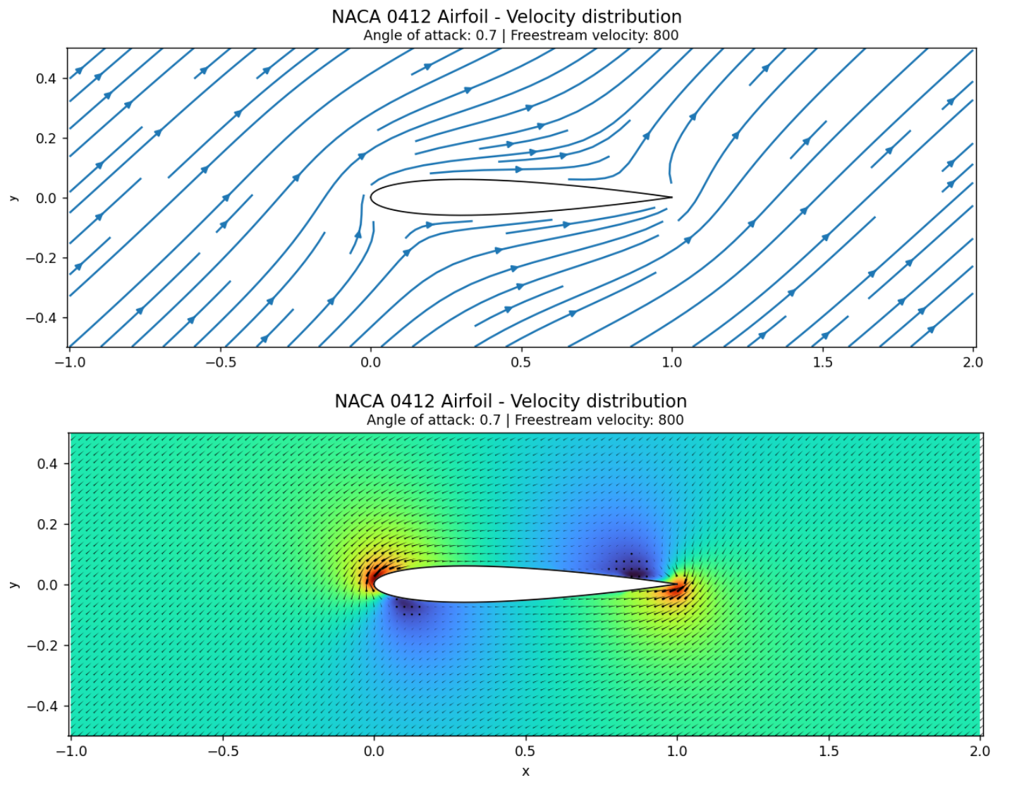
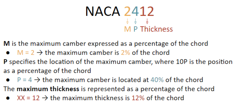
With our arrays of pressure and velocity at all points in the grid, this can be done easily with matplotlib:
naca_plot(nacadigits)
im = ax1.imshow(
speed_fine,
extent=[XXX.min(), XXX.max(), YYY.min(), YYY.max()],
origin="lower",
cmap="turbo",
interpolation="bilinear",
aspect="equal"
)
#plt.streamplot(XXX, YYY, U, V)
plt.quiver(XXX, YYY, U, V, headwidth=0.5)
plt.xlabel("x")
plt.ylabel("y")
plt.axis('equal')
#plt.grid(True)
plt.suptitle(f"NACA {nacadigits} Airfoil - Velocity distribution", fontsize=13)
plt.title(f"Angle of attack: {V_a} | Freestream velocity: {V_fs}", fontsize=10)
plt.show()
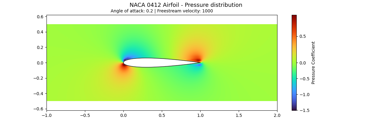
#PRESSURE DISTRIBUTION PLOT
rho = 1.225
P_inf = 0
P = P_inf + 0.5 * rho * (V_fs**2 - speed_fine**2)
Cp = 1 - (speed_fine / V_fs)**2
fig, ax = plt.subplots(figsize=(12,4))
cmap = plt.cm.turbo
#center the colormap at 0
norm = TwoSlopeNorm(vmin=np.min(Cp), vcenter=0, vmax=np.max(Cp))
im = ax.imshow(
Cp,
extent=[XXX.min(), XXX.max(), YYY.min(), YYY.max()],
origin="lower",
cmap=cmap,
norm=norm,
interpolation="bilinear",
aspect="equal"
)
plt.suptitle(f"NACA {nacadigits} Airfoil - Pressure distribution", fontsize=13)
plt.title(f"Angle of attack: {V_a} | Freestream velocity: {V_fs}", fontsize=10)
plt.colorbar(im, label='Pressure Coefficient')
naca_plot(nacadigits)
plt.axis('equal')
plt.show()And we are done!
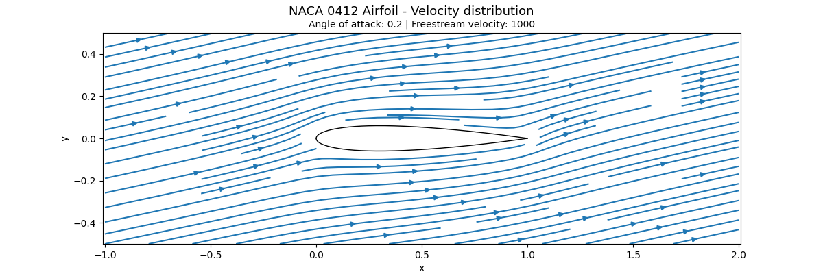
We can now run the program to produce plots like the ones below (for a NACA 0412 profile) at an angle of attack of 0.2 radians.
I really enjoyed this project; it was a lot of maths and physics theory I hadn’t covered yet but I loved going through the derivations and understanding where all the equations come from as well as implementing them. The program is able to plot cambered profiles and analyse their airflow (shown at the start) but I thought I would leave that out in the demonstration as technically this method does not work for cambered airfoils as they are asymmetric. Asymmetric flows have a non-zero circulation but sources on their own cannot result in any circulation and hence no lift. Regardless, I do plan to make a source-vortex panel method soon where I can experiment with more physically accurate methods for this visualisation.