Simulation

I began this project by simulating the movement of an inverted pendulum in Python to model the dynamics of the system before physically building the robot. As there are degrees of freedom (position and tilt angle), we’ll need two differential equations to model the system.

This step can be using either Newtonian mechanics (using forces) or Lagrangian mechanics (using energy). Below, I’ll be going through the derivation through Newtonian mechanics starting with basic force diagrams. These force diagrams will be created in the reference frame of the wheels and hence a psuedoforces are placed on the robot body (modelled as a rod) and the wheels respectively.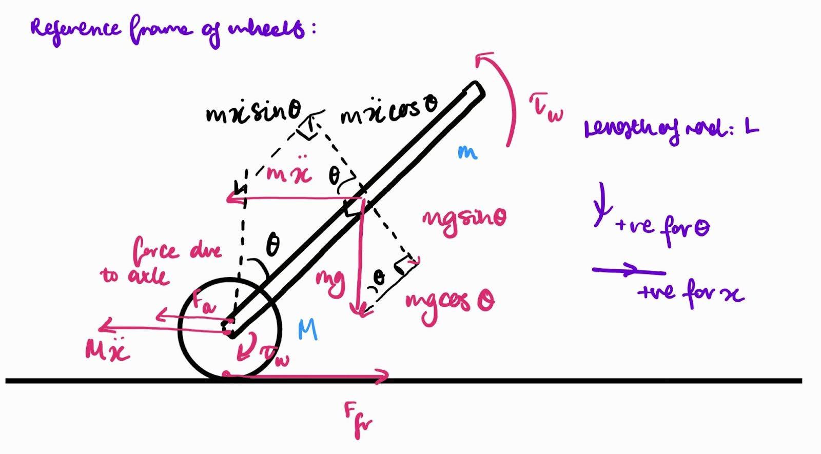

We’ll derive the first equation by equating the net torque on the rod with {the moment of inertia * angular acceleration}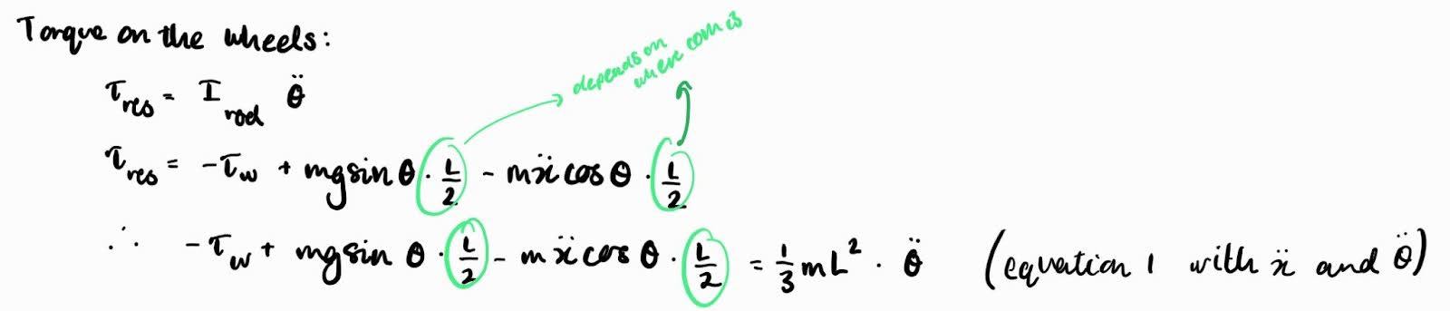

Our second equation will come from equating the net external force on the system with the acceleration of the centre of mass of the system.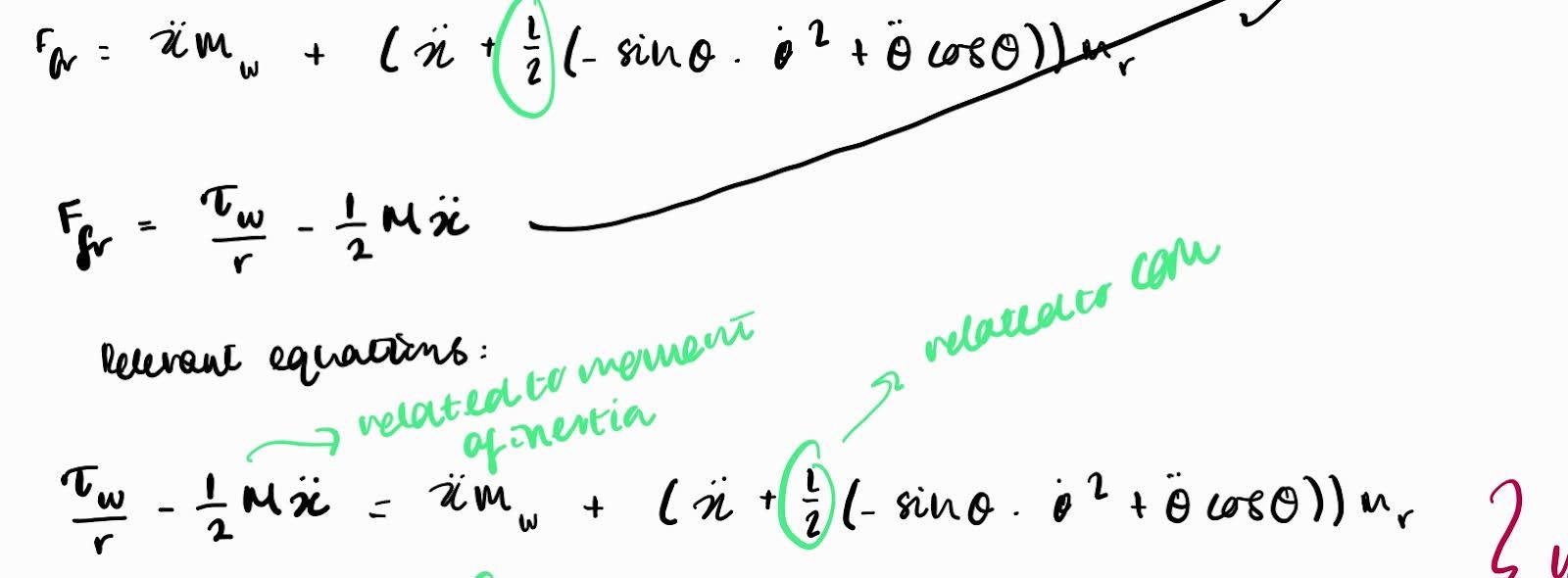

Now that we have our two equations, we rearrange the simultaneous equations to get equations with theta double dot and x double dot as the subject. Rearranging these equations is rather arduous manually, so we’ll use np.linalg to do this:

a = np.array ([[(self.length_rod*self.com*self.mass_rod*np.cos(theta)),(1/3*self.mass_rod*self.length_rod**2)],
                     [((3/2)*self.mass_wheel+self.mass_rod),(self.length_rod*self.com*self.mass_rod*np.cos(theta))]])
        b = np.array([(-torque_wheel+self.mass_rod*G*np.sin(theta)*self.length_rod*self.com),((torque_wheel/self.wheel_radius) + self.length_rod*self.com*self.mass_rod*np.sin(theta)*thetadot**2)])
       
        vals = np.linalg.solve(a,b)

Defining the state vector as x, xdot, theta and thetadot​​, we then apply numerical integration (SciPy’s solve_ivp) using the derived expressions and initial conditions, this yields the full state trajectory, from which we can analyse system behaviour over time.

Now we have values describing our state space at all points in time within our defined timeframe in terms of physical properties of our system such as moment of inertia of the robot, the mass of the wheels, mass of the robot, COM of the robot etc. However our equations contain one variable property: torque of the wheel. This is the variable that we apply our control system to. We'll begin with PID control.

PID Control

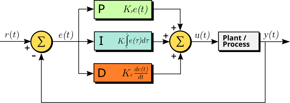
PID control is by far the most common feedback-based control algorithm for linear (systems for which the response is proportional to the input) and symmetric systems requiring continuous control. 

The basic principles of PID control is as follows: a PID controller continuously calculates the error as the difference between the setpoint (system’s desired state) and the process variable (current measured value). The controller then applies a correction torque to the robot scale based on the proportional, integral and derivative terms:

• Kp (proportional gain): Provides an immediate and proportional response to drive the system back to the setpoint. It is multiplied by the error e(t).
• Ki (integral gain): Prevents steady state error - the error that is present when time tends to infinity. It is multiplied by the accumulated error over time.
• Kd (derivative gain): Prevents overshooting and acts as a dampening term - for example when the error is quickly decreasing and approaching zero, this term increases thus preventing the overshooting. It is multiplied by the time derivative of the error.

Although PID is designed to work with linear systems, the actual dynamics of a self balancing robot are not linear as the angular acceleration depends on sin θ and cos θ terms. In practice, however, the system can be assumed to be linear about the upright position - this is something that we’ll explore further in equations in LQR control.

In two-wheeled self balancing robots, however, it is common to implement a PD controller instead of a full PID controller. We’ll omit the integral term as our system reacts quickly and the integral term tends to lag behind and hence it can accumulate a large error over time (integral windup) resulting in sudden overcorrections.

In our simulation, this is implemented by passing the state vector and the controller gains into the compute_torque function. This function then multiplies the corresponding parameters and then clips the torque, ensuring the max torque of the motors is not exceeded. The dynamics function then substitutes this value of torque_wheel into the differential equation to find theta double dot and x double dot. This yields the time derivative of the state vector at this time, which is then numerically integrated by solve_ivp.

    def _compute_torque(self, xdot, theta, thetadot, kp, ki, kd):
        torque_wheel = kp * theta + kd * thetadot #THIS IS WHAT GOES INTO THE SIMULATION
        torque_wheel = np.clip(torque_wheel, -self.motor.max_torque*2* self.motor_torque_safety_margin, self.motor.max_torque*2* self.motor_torque_safety_margin)
        #max_torque = self.motor.get_max_abs_torque(xdot / self.wheel_radius) * self.motor_torque_safety_margin
        #torque_wheel = np.clip(torque_wheel, -max_torque, max_torque)


        pwm = self.calculate_pwm(torque_wheel)


        return torque_wheel


    def dynamics(self, t, y, kp, ki, kd): # calculate the derivates and double derivates using differential equations
        x, xdot, theta, thetadot = y
        torque_wheel = self._compute_torque(xdot, theta, thetadot, kp, ki, kd)


        a = np.array ([[(self.length_rod*self.com*self.mass_rod*np.cos(theta)),(1/3*self.mass_rod*self.length_rod**2)],
                     [((3/2)*self.mass_wheel+self.mass_rod),(self.length_rod*self.com*self.mass_rod*np.cos(theta))]])
        b = np.array([(-torque_wheel+self.mass_rod*G*np.sin(theta)*self.length_rod*self.com),((torque_wheel/self.wheel_radius) + self.length_rod*self.com*self.mass_rod*np.sin(theta)*thetadot**2)])
       
        vals = np.linalg.solve(a,b)


        x2dot = vals[0]
        theta2dot = vals[1]


        ydot = [xdot, x2dot, thetadot, theta2dot]


        return ydot

Numerical integration:

    def run_simscipy(self, kp, ki, kd): # run the simulation using scipy
        solution = solve_ivp(self.dynamics, self.timespan, self.initialconditions, t_eval=self.time, args=(kp,ki,kd))
        print(solution.message)
        self.x = solution.y[0]
        self.xdot = solution.y[1]
        self.theta = solution.y[2]
        self.thetadot = solution.y[3]


        self.time = solution.t
        self.num_steps = len(self.time)

With our full state trajectory we can now simulate the dynamics of the robot in matplotlib which allows us to tune PID values. The typical way to do this is to turn the value of Kp up until it oscillates about its setpoint and then increase Kd until the robot stops overcorrecting.

Here's a snapshot from the working PID controller in simulation: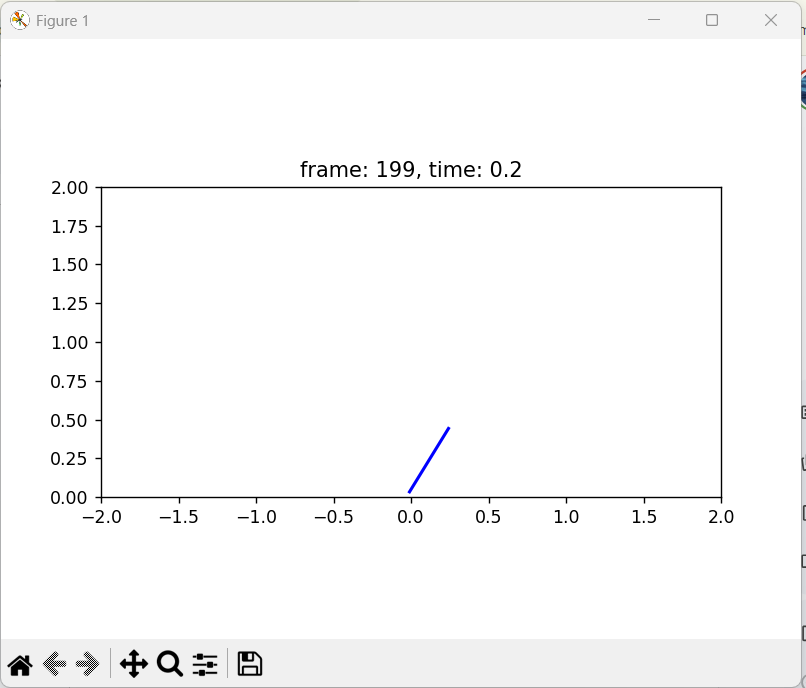

LQR Control

LQR control stands for linear quadratic regulator and it is a control algorithm that, unlike PID, is a state-space optimal control method. LQR calculates a gain matrix that minimizes a cost function combining error from the upright position and control effort. This allows for smoother and more efficient balancing compared to manually tuned PD controllers. The LQR method assumes linearised dynamics near the upright position, which is a valid approximation for small tilt angles.

In order to linear the dynamics I approximated sin theta as theta and cos theta as 1.

LQR control also has a Q matrix (matrix which describes how much you want to penalise error in each variable) and R which penalises controller effort. 

The A and B LQR matrices can be derived from the differential equations we made at the start.

import numpy as np
import control as ct


Q = np.diag([1, 3, 5, 5]) #2, 30, 5, 20
R = np.array([[7]])


A = np.array([[0, 1, 0, 0],[0, 0, -18.561, 0], [0, 0, 0, 1], [0, 0, 370.04, 0]])


B = np.array([[0],[134.795], [0], [-2034.736]])


print (ct.lqr(A, B, Q, R))

This now outputs our optimal gain matrix which we can apply to the motor’s torque by calculating the optimal gain matrix dotted with the state space.

Physical implementation

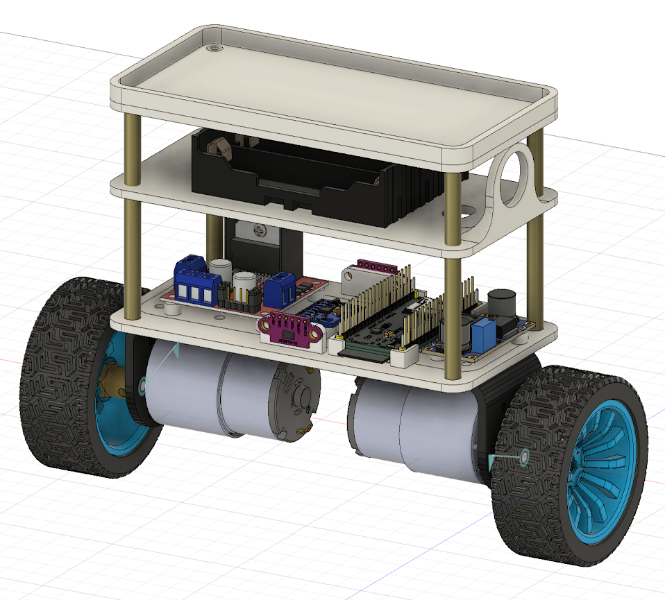
I designed a chassis in CAD, matching the simulation dimensions to ensure the centre of mass, rod length and wheel spacing were accurate.

The robot uses an IMU which combines:

• Accelerometer: Measures linear acceleration, which can be used to estimate tilt via gravity. The accelerometer gives a stable tilt estimate in the long term but is noisy, especially if the robot moves horizontally.
• Gyroscope: Measures angular velocity, which tells how fast the robot is rotating. The gyroscope gives smooth short-term angular velocity but drifts over time, accumulating error.

I used the angular velocity obtained from the gyroscope integrated over time along with the initial angle to get a gyroscopic estimate of the angle. Simultaneously, I used the orientation of the accelerometer’s data to get the accelerometer’s estimate of the angle. I implemented a complementary filter to fuse the gyroscope and accelerometer data, using a high-pass filter on the integrated gyroscope angle and a low-pass filter on the accelerometer. To reduce the effect of sensor noise, I applied a moving average over the last three computed angle values before using the result in the control loop.

Making process

In making the robot with PID, at the start I had many problems trying to get the robot to balance. It either fell weakly or oscillated erratically. Initially, I tried to reduce the delays between feedback loops; I did this by ensuring no redundant calculations throughout and ensuring no serial outputs during the loops. This helped and reduced the update time between loops which was much better. This did help but the main fix was changing the way that the torque was mapped to the PWM. I had initially carried out an experiment to calculate the amount of torque that each PWM on my motors correspond to by seeing the amount of weight the motors could lift with a pulley. When I plotted the data I got from this, the data looked like a quadratic regression and hence this is what I had initially applied to the program. I didn’t realise until much later however that this was the issue in my balancing. While toying around with the system, I changed the regression to a linear one, assuming that maybe I was overfitting some inaccuracies in my experimental data which was causing problems. This instantly fixed the problem and the robot reached a state that made it manageable to slightly tweak values and result in smooth balancing. In retrospect, this was an expected fix and PID and LQR are both control algorithms that work on linear programs.

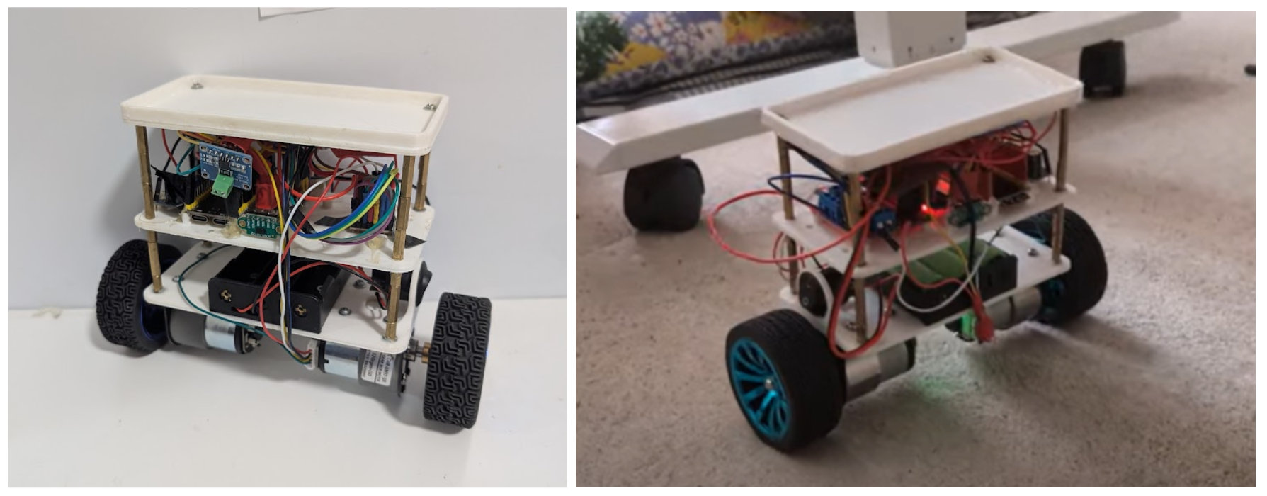
In the end my robot came out looking like this and balancing quite smoothly, recovering from perturbations automatically.

Video of balancing: https://youtu.be/UXDT873h59I

Building this robot was a full-cycle project: from simulating the dynamics in Python, to designing the LQR controller to filtering real sensor data. It was extremely fun and a great insight into the topic of control systems which I hadn’t delved into before.